ECE :: Automatic Control Systems
-
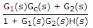
The compensator in the given figure is a

-
If G(s) H(s) =
 , the closed loop poles are on
 -
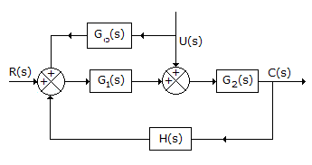
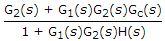
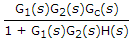
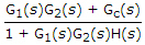
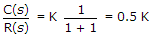
For the block diagram of the given figure, the equation describing system dynamics is
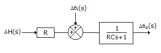
-
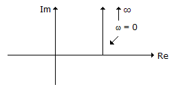
The polar plot of
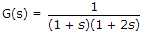
-
In a second order undamped system, the poles are on
-
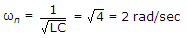
For the system of the given figure, the undamped natural frequency of closed loop poles is
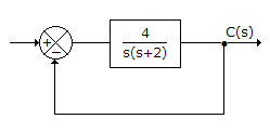
-
An open loop system has a forward path transfer function (42.25)/s(s + 6.5). The unit step response of the system starting from rest will have its maximum value at a time equal to


 Whatsapp
 Facebook


 to give AQ0(s).
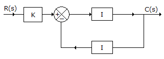
 .
. .
.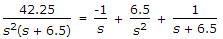 Taking inverse transform, the time domain response is - 1 + 6.5t + e-6-5t. It reaches maximum value at t = infinity.